Vanila Implementation of Python and Data-Modeling in Financial markets.
Python LInked-lists.
Python Stacks and Queues.
Python BinarySearch Trees.
Python HashTables.
Vanila Implementation of Python and Data-Modeling in Financial markets.
Python LInked-lists.
Python Stacks and Queues.
Python BinarySearch Trees.
Python HashTables.
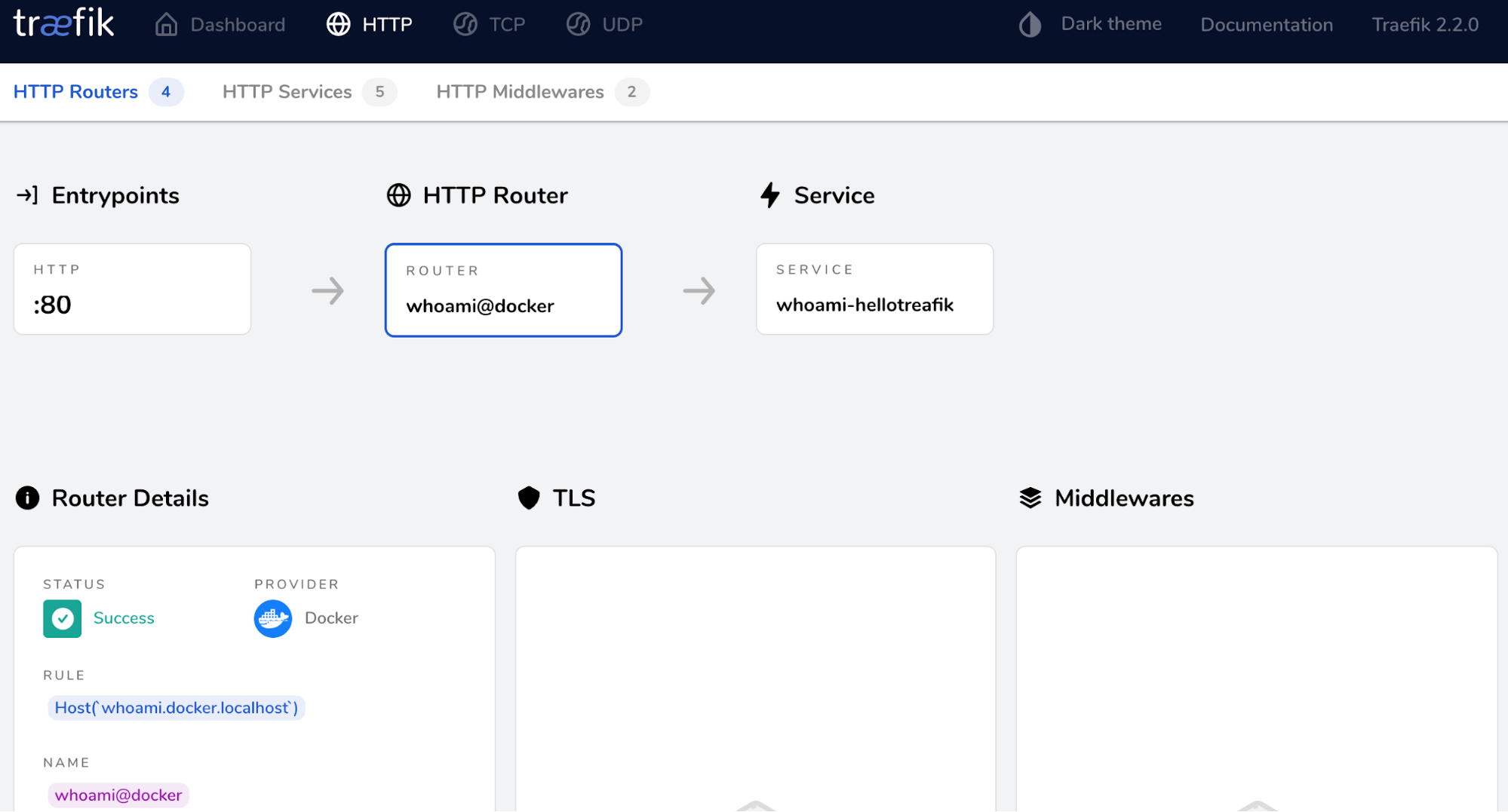
Service Discovery:
Default Dash-Board

InBuilt Authentication,Http Connection handling(timeout and etc) For EntryPoints and MiddleWares.
More UI Features:
Configuration For EntryPoints and Routers
https://docs.traefik.io/providers/overview/
Consul Example:
[providers.consul]
endpoints = [“127.0.0.1:8500”]
rootKey = “traefik”
ETCD example:
[providers.etcd]
endpoints = [“127.0.0.1:2379”]
rootKey = “traefik”
Full Path Details for Keys and Values
https://docs.traefik.io/routing/providers/kv/
Routers:
Entry Points talks to Routes to Call out Service Functions/Routes.
*Full Regex Support with && || conditions
* Priority Can be assigned to Each Route.
[http.routers]
[http.routers.Router-1]
rule = “HostRegexp(`.*\.traefik\.com`)”
# …
[http.routers.Router-2]
rule = “Host(`foobar.traefik.com`)”
Source: https://docs.traefik.io/routing/routers/
Available Configuration Options:
https://docs.traefik.io/routing/providers/kv/
Health Checks:
It keeps doing health checkups of services, and are considered alive as long as they reply back with 2xx, 3xx HTTP codes
Mirroring:
My Docker command:
docker run -d --name timescaledbworks -p 5000:5432 -e POSTGRES_PASSWORD=test -e POSTGRES_USER=test -e POSTGRES_DB=test timescale/timescaledb:latest-pg11
my GoLnag Source:
package main
import (
"database/sql"
_ "github.com/lib/pq"
"fmt"
)
func main() {
var err error
// test without port thing
connStr := "user=test dbname=test password=test host=0.0.0.0 sslmode=disable port=5000"
db, err := sql.Open("postgres", connStr)
if err != nil {
fmt.Println("could not connecet to Daatabase")
}
fmt.Println(db)
if err := db.Ping(); err != nil {
fmt.Println("unable to ping DB : " + err.Error())
return
}
//else{
//fmt.Println("able to connecet to db")
//}
//db.Query("CREATE TABLE conditions(time TIMESTAMP NOT NULL,location TEXT NOT NULL,temperature DOUBLE PRECISION NULL,humidity DOUBLE PRECISION NULL);")
//db.Query("CREATE EXTENSION IF NOT EXISTS timescaledb CASCADE;")
//db.Query("CREATE TABLE hello")
//db.Query("SELECT create_hypertable('conditions','time','location',4);")
}
When you don’t want to type username an password each time or when you are not allowed to do so as well.
Your repo should look like this:
git@github.com:USERNAME/REPOSITORY.git
you can see config using:
nano .git/config
SSH key can be generated like:
ssh-keygen -t rsa -b 4096 -C “arshpreet.singh@myemail.com”
More about Git and adding ssh key can be found here:
https://help.github.com/articles/connecting-to-github-with-ssh/
This is an Easy to do things in python so we can run scripts using command line Arguments for us as well.
import click

@click.command()
@click.option('--count',default = 1, )
@click.option('--name',prompt = "What you are supposed to do here?")
def test_click(count,name):
    for i in range(count):
        click.echo(str(name))
'''
How to run this script:

python test_click.py --name "Arsh" --count 4

'''
This is Python Script that you can use to send Messages on any Phone without leaving trace of any number.
# python script for sending message update

import time
from time import sleep
from sinchsms import SinchSMS

# function for sending SMS
def sendSMS():

	# enter all the details
	# get app_key and app_secret by registering
	# a app on sinchSMS
	number = '+919915959387'
	app_key = '29d0e101-e619-4226-823a-c39c4b99b5ac'
	app_secret = '1WkUjJ3RWEy1P9h9mw/2sQ=='

	# enter the message to be sent
	message = "hello"

	client = SinchSMS(app_key, app_secret)
	print("Sending '%s' to %s" % (message, number))

	response = client.send_message(number, message)
	message_id = response['messageId']
	response = client.check_status(message_id)

	# keep trying unless the status retured is Successful
	while response['status'] != 'Successful':
		print(response['status'])
		time.sleep(1)
		response = client.check_status(message_id)

	print(response['status'])

if __name__ == "__main__":
	sendSMS()
Falcon framework is great when you have to build micro-services in Python, All we need to do is create a Class that would provide the specific Purpose to Establish one Micro-service as Route and add the route to the API would be able to server as deploy multiple modes inside the Falcon Architecture as well.
# sample.py
import falcon
class QuoteResource:
def on_get(self, req, resp):
"""Handles GET requests"""
quote = {
'quote': (
"I've always been more interested in "
"the future than in the past."
),
'author': 'Grace Hopper'
}
resp.media = quote
class HelpObject:
def on_get(self, req, resp):
"""Handles GET requests"""
quote = {
'quote': (
"I've always been more interested in "
"the future than in the past."
),
'author': 'Arshpreet Singh'
}
resp.media = quote
api = falcon.API()
api.add_route('/quote', QuoteResource())
api.add_route('/quote2', HelpObject())
<span id="mce_SELREST_start" style="overflow:hidden;line-height:0;"></span>
model/*.cto file- This file is able to describe Asset, Participant and Transactions those occur at that business network as well .
If your model is very large, you can have multiple .cto model files, as necessary. Every .cto model file must include a single namespace and at least one resource definition.
NameSpace: NameSpace is just naming convention for the File-System. For each of your .cto file namespace would be an unique name for the file. Each of the resources available in the file would be taken from that namespace.
Resource: Now we have following kind of resources we can use.
Asset: A business network Asset(Example Bit-coin is an Asset in Bit-coin-Network)
Transaction: A business Logic
Participant: A business network Participant
Event: Notification of something happening in the network
Enumerated Type: A set of named Values
Concept: Any object you want to model that is not one of the other types
Each resource type corresponds to its model type of the same name (for example, asset is used to model an Asset, participant models a Participant, etc.)
asset Vehicle identified by vehicle_id {
}
Week4_DataF
# Import the required packages
using Distributions, DataFrames
# Seed the random number generator
srand(1234);
# Question 4: Create the 3 x 30 array named array_1
# 30 rows and 3 columns array
array_1 = [rand(30) rand(30) rand(30)]
size(array_1)
array_1
# Question 5: Mean and variance of column 1
mean_column_1 = mean(array_1[:,1])
var_column_1=var(array_1[:,1])
println("mean=",mean_column_1)
println("var=",var_column_1)
# Question 5 (continued): Mean and variance of column 2
mean_column_2 = mean(array_1[:,2])
var_column_2=var(array_1[:,2])
println("mean=",mean_column_2)
println("var=",var_column_2)
# Question 5 (continued): Mean and variance of column 3
mean_column_3 = mean(array_1[:,3])
var_column_3=var(array_1[:,3])
println("mean=",mean_column_3)
println("var=",var_column_3)
# Question 6: Import array_1 into a DataFrame named df
df = DataFrame(array_1)
# check available names and fieldnames in Julia, Python's alternative
f_name =fieldnames(df)
name=names(df)
println(f_name,name)
# Accessing different columns of df
df[:x3]
# Question 7: Change the names of the columns to Var1, Var2, and Var3
rename!(df,Dict(:x1=>:Var1,:x2=>:Var2,:x3=>:Var))
### we can also tail function see last required entries
tail(df,20)
# Creatring Second DataFrame
df2=DataFrame(tail(df,20))
# Question 9: Calculate simple descriptive statistics of all the columns in df2 using the describe() function
describe(df2)
# Question 10: Add a column to df2 named Cat1 to df2 consisting of randomly selecting either the strings GroupA or GroupB
df2 = hcat(df2, rand(["GroupA","GroupB"],20))
rename!(df2,Dict(:x1=>:Cat1))
# Question 11: Create a new DataFrame named df3
df3 = DataFrame(A=1:20,B=21:40,C=41:60)
# Question 12: Change indicated values to empty entries
#In a code cells below, change the values in df3 of the following cells to NA: row 10, column 1, row 15, column 2 and row #19, column 3
df3[10,1] = NA
df3[15,2] = NA
df3[19,3] = NA
df3
# Question 13: Create DataFrame df4 that contains no rows with NaN (NA) values
df4 = completecases!(df3)
Week3_PR_Template
# Initilization of Plots Package
using Plots
pyplot()
data_tofit = readdlm("Week3_PR_Data.dat", '\t', header=true)
typeof(data_tofit)
new_array=data_tofit[1]
for i in 1:size(new_array)[1]
    println(new_array[i,:])
end
# Create the arrays x and y, assigning x the first column of data_tofit and y the second column
x,y = new_array[:,1],new_array[:,2]
scatter(x,y)
# Create a function called parabfit, with x as the argument, returning a*x^2 + b*x + c
parabfit(x)=a*x^2 + b*x + c
a = 1
b = 1
c = 1

plot(parabfit,-2,2)
# Create variables a, b and c, assigning each the value 1
a = 1
b = 1
c = 1

# Plot the function parabfit, for x values between -5 and 5
plot(parabfit,-5,5)
# More plot!() tries.
a,b,c = 1,1,1
scatter(x_axis,y_axis)
plot!(parabfit,-5,5)
Optimize parameters a, b and c such that it fits the data points more concisely.
# More plot!() tries.
a,b,c = -1,2,3
scatter(x,y)
plot!(parabfit,-5,5)
# More plot!() tries.
a,b,c = -1,0.1,2
scatter(x_axis,y_axis)
plot!(parabfit,-5,5)
# More plot!() tries.
a,b,c = -1,0.8,3
scatter(x,y)
plot!(parabfit,-5,5)
# More plot!() tries.
a,b,c = -0.9,2.7,0.05
scatter(x,y)
plot!(parabfit,-5,5)
a,b = 1,1
plot(scatter(x,y,alpha=0.5))
c=0
plot!(parabfit,-5,5)
c = -1
plot!(parabfit,-5,5)
c = -2
plot!(parabfit,-5,5)
c = -3
plot!(parabfit,-5,5)
c = -4
plot!(parabfit,-5,5)
c = -5
plot!(parabfit,-5,5)
c = 2
plot!(parabfit,-5,5)
c,b = 1,1
plot(scatter(x,y,alpha=0.5))
a=0
plot!(parabfit,0,5)
a = -1
plot!(parabfit,0,5)
a = -2
plot!(parabfit,0,5)
a = -3
plot!(parabfit,0,5)
a = -4
plot!(parabfit,0,5)
a = -5
plot!(parabfit,0,5)
a = 2
plot!(parabfit,0,5)
#Locating final value for a
c,b = 3,1
plot(scatter(x,y,alpha=0.5))
a = -1
plot!(parabfit,0,5)
c,a = 2,-1
plot(scatter(x,y,alpha=0.5))
b=0
plot!(parabfit,0,5)
b = 1
plot!(parabfit,0,5)
b = 2
plot!(parabfit,0,5)
b = 3
plot!(parabfit,0,5)
b = 4
plot!(parabfit,0,5)
b = 5
plot!(parabfit,0,5)
b = -1
plot!(parabfit,0,5)
# plotting for b=4
c,a = 1,-1
plot(scatter(x,y,alpha=0.5))
b = 3
plot!(parabfit,0,8)
# plotting for b=4
c,a,b = 1,-1,3
plot(scatter(x,y,alpha=0.5))
plot!(parabfit,0,5)
To optimize values of a,b,c we had to plot one variable many times to find out one variable’s occurrence at different levels
of scale. By changing the range of parabola function it was more easy to come up with more accurate values of a,b and c